# 鋭い Nash の不等式と L¹ の罰金つき Dirichlet 汎関数：Carlen–Loss の定数・最小化子・尺度則

> Nash の不等式を Fourier 変換で示し、3 次元の鋭い定数を対称減少再配置と球の動径 Neumann 問題で求める（Carlen–Loss）。汎関数 ½‖∇u‖²+γ‖u‖₁ の最小値の尺度則と閉じた形、劣加法性、定数の区間演算による包含も示す。
> https://rikai.mugen-giken.com/mathematics/pde/sharp-nash-inequality

## 0. この記事の要点

関数の「大きさ」の測り方はいくつもあります。総量（$L^1$ ノルム）、二乗の総量（$L^2$ ノルム）、そして傾きの二乗の総量（勾配の $L^2$ ノルム）です。総量が決まっていて傾きも小さい関数は、高く尖ることも薄く広がりすぎることもできないので、二乗の総量も小さくなるはずです。この直観を不等式にしたのが Nash の不等式で、この記事ではその最良の定数と、最良の定数を与える関数（最適化子）を 3 次元で求めます。

- **Nash の不等式** $\lVert f\rVert_2^{2+4/d}\le C\lVert\nabla f\rVert_2^2\lVert f\rVert_1^{4/d}$ は、Fourier 変換で低い周波数と高い周波数に分けるだけで示せます（任意の次元 $d$）。
- 3 次元の**最良の定数**は $C_{\mathrm N}=\frac{5^{5/3}}{2^{2/3}\cdot3\,x_1^2(4\pi/3)^{2/3}}=0.05851\ldots$ です。$x_1=4.4934\ldots$ は $\tan x=x$ の最小の正の根で、球の動径方向の Neumann 問題の最初の $0$ でない固有値 $x_1^2$ として現れます。証明は対称減少再配置と、球の上の動径関数の Poincaré の不等式の組み合わせです（Carlen–Loss）。
- 最適化子は $u(x)=\bigl(1-\frac{\sin\lvert x\rvert}{\lvert x\rvert\cos x_1}\bigr)_+$ で、半径 $x_1$ の球の外で $0$、境界で値も傾きも $0$ になる $C^1$ 関数です。
- $L^1$ の罰金つき Dirichlet 汎関数 $\mathcal E_\gamma[u]=\frac12\lVert\nabla u\rVert^2+\gamma\lVert u\rVert_1$ の質量 $\lVert u\rVert_2^2=\theta$ での最小値は $\theta^{5/7}\gamma^{4/7}F[1]$ で、$F[1]=\frac74(\frac2{3C_{\mathrm N}})^{3/7}=4.9646157\ldots$ です。$\theta^{5/7}$ は強い劣加法性を持ち、質量を分けるとエネルギーが必ず上がります。
- $x_1$、$C_{\mathrm N}$、$F[1]$ は区間演算で小数 30 桁まで包含します（計算機援用の命題、コードつき）。

## 1. 動機

Nash は 1958 年の論文で、係数が滑らかでない放物型方程式 $\partial_tu=\nabla\cdot(a\nabla u)$ の解が Hölder 連続であることを示しました。その出発点がこの記事の不等式で、熱の総量 $\lVert u\rVert_1$ が保存されるという事実と組み合わせると、解の $L^2$ ノルムが $t^{-d/4}$ の速さで減衰することが係数の滑らかさによらずに出ます（<Ref to="ex-nash-heat" />）。ほぼ同じ時期に De Giorgi も楕円型方程式について独立に同種の結果を得ており、両者の方法は今日の楕円型・放物型方程式の正則性理論の土台になっています。

不等式の形は尺度で決まります。$f$ を $\lambda f(\mu x)$ に置き換えると両辺が同じ倍率で変わるのは、指数が $2+\frac4d$ と $\frac4d$ の組のときだけです（<Ref to="exr-nash-exponents" />）。定数の最良値は長く知られていませんでしたが、Carlen と Loss は 1993 年に、対称減少再配置で問題を球対称な関数に帰着し、球の中と外を分けて評価することで、最良の定数とそれを与える関数を求めました。その鍵は、球の上の動径関数の Poincaré の不等式の最良の定数が、球の Neumann 問題の動径方向の最初の固有値で決まることです。

後半では、同じ定数が変分問題
$$
\inf\Bigl\{\frac12\lVert\nabla u\rVert_2^2+\gamma\lVert u\rVert_1:\lVert u\rVert_2^2=\theta\Bigr\}
$$
の最小値を決めることを見ます。運動エネルギー $\frac12\lVert\nabla u\rVert^2$ は $u$ を広げようとし、$\gamma\lVert u\rVert_1$ は $u$ を狭い範囲に集めようとします（質量 $\theta$ を固定すると、$L^1$ ノルムは関数が集中しているほど小さい）。この釣り合いは Thomas–Fermi 型の平均場の汎関数の簡単な例で、Bach–Hach（2022）は量子電磁力学の非相対論的な模型（Pauli–Fierz 模型）で切断を大きくする極限を調べるために、この汎関数を比較の対象として導入しました。最小値の尺度則・閉じた形・劣加法性は、こうした応用で「エネルギーが最小に近い配位はどんな形か」を論じるときの基本的な道具になります。

## 2. 準備

この記事で使う事前知識は次のとおりです。

- 対称減少再配置 $f^*$ とその性質（[対称減少再配置](/mathematics/pde/dirichlet-laplacian-weyl-law#def-symmetric-rearrangement)、<Ref to="mathematics/pde/dirichlet-laplacian-weyl-law#lem-rearrangement-basic" />）と Pólya–Szegő の不等式（<Ref to="mathematics/pde/dirichlet-laplacian-weyl-law#thm-polya-szego" />）。
- Fourier 変換と Plancherel の定理（[Fourier 変換](/mathematics/fourier-analysis/fourier-transform)）、$H^1(\mathbb R^d)$ の Fourier による特徴づけ（<Ref to="mathematics/fourier-analysis/sobolev-spaces#prop-hk-wk2" />）。
- 軟化と $H^1$ での近似（<Ref to="mathematics/fourier-analysis/sobolev-spaces#thm-density" />）。
- 区間演算の包含原理と区間 Newton 法（[浮動小数点と区間演算](/mathematics/computer-assisted-proofs/floating-point-interval-arithmetic)）。
- $W^{1,\infty}$ の関数との積と区分的に滑らかな切り落とし（<Ref to="mathematics/pde/box-neumann-tools#lem-product-rule" />、<Ref to="mathematics/pde/box-neumann-tools#lem-tensor-cutoff" />）。

### 2.1. 記号

| 記号 | 意味 |
|---|---|
| $\lVert f\rVert_p$ | $L^p(\mathbb R^d)$ ノルム。$\lVert\nabla f\rVert_2^2=\int\lvert\nabla f\rvert^2$ |
| $\omega_d=\lvert B_1\rvert$ | 単位球の体積（$\omega_3=4\pi/3$） |
| $\mathcal N_d(f)=\lVert f\rVert_2^{2+4/d}/(\lVert\nabla f\rVert_2^2\lVert f\rVert_1^{4/d})$ | Nash の比 |
| $x_1\in(\pi,\frac32\pi)$ | $\tan x=x$ の最小の正の根、$x_1=4.4934\ldots$ |
| $C_{\mathrm N}=\frac{5^{5/3}}{2^{2/3}\cdot3\,x_1^2(4\pi/3)^{2/3}}$ | 3 次元の鋭い Nash の定数 |
| $u(x)=\bigl(1-\frac{\sin\lvert x\rvert}{\lvert x\rvert\cos x_1}\bigr)\mathbf 1_{\lvert x\rvert\le x_1}$ | 最適化子 |
| $\mathcal E_\gamma[u]=\frac12\lVert\nabla u\rVert_2^2+\gamma\lVert u\rVert_1$ | $L^1$ の罰金つき Dirichlet 汎関数（$\gamma\gt0$） |
| $E_{\mathrm{MF}}(\theta;\gamma)$ | 質量 $\lVert u\rVert_2^2=\theta$ での $\mathcal E_\gamma$ の下限 |
| $F[\beta]=E_{\mathrm{MF}}(1;\beta)$ | Bach–Hach の比較の汎関数の最小値。$F[1]=4.9646\ldots$ |

文献との対応: Carlen–Loss は $d$ 次元の最良の定数を $C_d$ と書き、3 次元では $C_3=C_{\mathrm N}$ です。Bach–Hach は $\mathcal F_\beta(\phi)=\frac12\lVert\nabla\phi\rVert^2+\beta\lVert\phi\rVert_1$ と書き、その $\lVert\phi\rVert_2=1$ での下限を $F[\beta]$ と書きます。この記事の $\mathcal E_\gamma$ と同じものです。

<Lemma id="lem-rearrangement-l1" title="再配置は L¹ ノルムを保つ">
可測関数 $f\ge0$ が $f\in L^1(\mathbb R^d)$ を満たせば、すべての $t\gt0$ で $\lvert\{f\gt t\}\rvert\lt\infty$ で、$\lVert f^*\rVert_1=\lVert f\rVert_1$ である。
</Lemma>

<Proof of="lem-rearrangement-l1">
Chebyshev の不等式から $\lvert\{f\gt t\}\rvert\le t^{-1}\lVert f\rVert_1\lt\infty$ です。Tonelli の定理（<Ref to="mathematics/real-analysis/product-measures-fubini#thm-tonelli" />）から $\int f=\int_0^\infty\lvert\{f\gt t\}\rvert\,dt$ で、<Ref to="mathematics/pde/dirichlet-laplacian-weyl-law#lem-rearrangement-basic" /> の 1 から $\lvert\{f^*\gt t\}\rvert=\lvert\{f\gt t\}^*\rvert=\lvert\{f\gt t\}\rvert$ なので、$f^*$ についても同じ値です。
</Proof>

## 3. Nash の不等式

<Theorem id="thm-nash-fourier" title="Nash の不等式">
$d\ge1$ とし、$C_d'=\bigl(1+\frac2d\bigr)^{1+2/d}\bigl(\frac d2\bigr)^{2/d}\bigl((2\pi)^{-d}\omega_d\bigr)^{2/d}$ とおく。すべての $f\in H^1(\mathbb R^d)\cap L^1(\mathbb R^d)$ について
$$
\lVert f\rVert_2^{2+4/d}\le C_d'\,\lVert\nabla f\rVert_2^2\,\lVert f\rVert_1^{4/d} .
$$
</Theorem>

<Proof of="thm-nash-fourier">
$f\in L^1\cap L^2$ なので、$L^1$ の意味の Fourier 変換 $\hat f$ は Plancherel の定理（<Ref to="mathematics/fourier-analysis/fourier-transform#thm-plancherel" /> の 1）の $L^2$ の Fourier 変換と一致し、$\lVert f\rVert_2^2=(2\pi)^{-d}\int\lvert\hat f\rvert^2$ です。また $\lvert\hat f\rvert\le\lVert f\rVert_1$（<Ref to="mathematics/fourier-analysis/fourier-transform#prop-ft-basic" /> の 1）、$\lVert\nabla f\rVert_2^2=(2\pi)^{-d}\int\lvert\xi\rvert^2\lvert\hat f\rvert^2$（<Ref to="mathematics/fourier-analysis/sobolev-spaces#prop-hk-wk2" /> と <Ref to="mathematics/fourier-analysis/sobolev-spaces#def-hs" />）です。$\rho\gt0$ で周波数を分けると
$$
\lVert f\rVert_2^2=(2\pi)^{-d}\Bigl(\int_{\lvert\xi\rvert\le\rho}+\int_{\lvert\xi\rvert\gt\rho}\Bigr)\lvert\hat f\rvert^2\le(2\pi)^{-d}\omega_d\rho^d\lVert f\rVert_1^2+\rho^{-2}\lVert\nabla f\rVert_2^2
$$
です。$A=(2\pi)^{-d}\omega_d\lVert f\rVert_1^2$、$B=\lVert\nabla f\rVert_2^2$ とおきます。$B=0$ なら $\hat f$ は $\xi\ne0$ でほとんど至るところ $0$ なので $f=0$ で、不等式は自明です。$B\gt0$ なら $\rho^{d+2}=2B/(dA)$ と選ぶと右辺は $(1+\frac2d)B\rho^{-2}=(1+\frac2d)B^{d/(d+2)}(\frac{dA}2)^{2/(d+2)}$ で、両辺を $\frac{d+2}d$ 乗すれば主張です。
</Proof>

$d=3$ では $C_3'=(5/3)^{5/3}(3/2)^{2/3}(\frac{4\pi/3}{8\pi^3})^{2/3}\approx0.2021$ で、§5 の最良の定数 $C_{\mathrm N}\approx0.0585$ の約 $3.5$ 倍です。Fourier による証明では、$\lvert\hat f\rvert\le\lVert f\rVert_1$ が全周波数で等号になる関数（デルタ関数）と、高い周波数だけに重みのある関数という、両立しない 2 つの極端を同時に使っているので、定数に損が出ます。

<Example id="ex-nash-heat" title="熱の L¹ から L² への減衰">
$f\ge0$ を滑らかで速く減衰する関数とし、$w(t)=e^{t\Delta}f$（熱方程式 $\partial_tw=\Delta w$ の解）を考えます。$w\ge0$ で総量 $\lVert w(t)\rVert_1=\lVert f\rVert_1$ は保存されます（[熱方程式](/mathematics/pde/heat-equation)）。$E(t)=\lVert w(t)\rVert_2^2$ とおくと $E'=2\mathrm{Re}\langle w,\Delta w\rangle=-2\lVert\nabla w\rVert_2^2$ で、Nash の不等式から $\lVert\nabla w\rVert_2^2\ge C^{-1}E^{1+2/d}\lVert f\rVert_1^{-4/d}$ です。よって $\frac{d}{dt}E^{-2/d}=-\frac2dE^{-1-2/d}E'\ge\frac4{dC}\lVert f\rVert_1^{-4/d}$ で、積分すると
$$
\lVert e^{t\Delta}f\rVert_2\le\Bigl(\frac{dC}{4t}\Bigr)^{d/4}\lVert f\rVert_1
$$
を得ます。$d=3$、$C=C_{\mathrm N}$ では $(3C_{\mathrm N}/4)^{3/4}t^{-3/4}\approx0.0959\,t^{-3/4}$ で、$f$ を点に集めた極限（熱核そのもの、$\lVert e^{t\Delta}\delta\rVert_2=(8\pi t)^{-3/4}\approx0.0891\,t^{-3/4}$）と 8% しか違いません。この議論は係数 $a(x)$ つきの方程式でもそのまま通ることが、Nash の方法の要点です。
</Example>

## 4. $\tan x=x$ の根と球の動径 Neumann 問題

<Lemma id="lem-root-x1" title="tan x = x の最小の正の根">
$g_0(x)=\sin x-x\cos x$ とおく。$g_0$ は $(0,\pi]$ で正、$[\pi,2\pi]$ で狭義減少で、$(\pi,\frac32\pi)$ にただ 1 つの零点 $x_1$ をもつ。$(0,x_1)$ で $g_0\gt0$ で、$x_1$ は $\tan x=x$ の最小の正の根である。
</Lemma>

<Proof of="lem-root-x1">
$g_0(0)=0$、$g_0'(x)=x\sin x$ です。$(0,\pi)$ で $g_0'\gt0$ なので $g_0\gt0$（$(0,\pi]$ 上）、$(\pi,2\pi)$ で $g_0'\lt0$ なので $g_0$ は $[\pi,2\pi]$ で狭義減少です。$g_0(\pi)=\pi\gt0$、$g_0(\frac32\pi)=-1\lt0$ なので、中間値の定理（<Ref to="mathematics/calculus/limits-and-continuity#thm-ivt" />）と狭義単調性から $(\pi,\frac32\pi)$ に零点がただ 1 つあり、$(0,x_1)$ では $g_0\gt0$ です。$\cos x\ne0$ の点では $\tan x=x$ と $g_0(x)=0$ は同値で、$(0,\frac\pi2)$ では $\tan x\gt x$（$g_0\gt0$）、$(\frac\pi2,\pi]$ では $\tan x\le0\lt x$ なので、$x_1$ より小さい正の根はありません。
</Proof>

<Figure caption="y = tan x と y = x。原点の次の交点が x₁ ≈ 4.4934 で、3π/2 ≈ 4.712 のすぐ手前にある。">
<svg viewBox="0 0 480 290" width="100%" role="img" aria-label="y = tan x と y = x のグラフ。0 から 3π/2 までに、原点以外では x₁ ≈ 4.4934 でだけ交わる。π/2 と 3π/2 に漸近線がある">
  <line x1="50" y1="212" x2="460" y2="212" stroke="currentColor" stroke-width="1" />
  <line x1="50" y1="15" x2="50" y2="262" stroke="currentColor" stroke-width="1" />
  <line x1="175.7" y1="15" x2="175.7" y2="262" stroke="currentColor" stroke-width="0.8" stroke-dasharray="4 4" opacity="0.6" />
  <line x1="427.0" y1="15" x2="427.0" y2="262" stroke="currentColor" stroke-width="0.8" stroke-dasharray="4 4" opacity="0.6" />
  <g font-size="12" fill="currentColor">
    <text x="166" y="280">π/2</text><text x="296" y="230">π</text><text x="414" y="280">3π/2</text><text x="464" y="216">x</text>
  </g>
  <line x1="301.3" y1="208" x2="301.3" y2="216" stroke="currentColor" />
  <polyline fill="none" stroke="var(--sl-color-accent)" stroke-width="2.2" points="50.0,212.0 53.0,211.1 55.9,210.2 58.9,209.3 61.9,208.4 64.8,207.5 67.8,206.6 70.8,205.6 73.7,204.7 76.7,203.7 79.7,202.7 82.6,201.6 85.6,200.6 88.6,199.4 91.5,198.3 94.5,197.1 97.5,195.8 100.4,194.5 103.4,193.1 106.4,191.6 109.3,190.0 112.3,188.3 115.3,186.5 118.2,184.5 121.2,182.4 124.2,180.0 127.1,177.4 130.1,174.5 133.1,171.3 136.0,167.6 139.0,163.3 142.0,158.4 144.9,152.6 147.9,145.6 150.9,137.0 153.8,126.2 156.8,112.0 159.8,92.7 162.7,64.6 165.7,20.0" />
  <polyline fill="none" stroke="var(--sl-color-accent)" stroke-width="2.2" points="212.8,260.0 215.3,256.4 217.9,253.1 220.5,250.2 223.1,247.6 225.7,245.2 228.3,243.1 230.9,241.1 233.4,239.2 236.0,237.5 238.6,235.9 241.2,234.4 243.8,233.0 246.4,231.7 249.0,230.4 251.5,229.2 254.1,228.1 256.7,227.0 259.3,225.9 261.9,224.9 264.5,223.9 267.1,223.0 269.6,222.0 272.2,221.1 274.8,220.3 277.4,219.4 280.0,218.6 282.6,217.7 285.2,216.9 287.7,216.1 290.3,215.3 292.9,214.5 295.5,213.7 298.1,213.0 300.7,212.2 303.3,211.4 305.8,210.6 308.4,209.9 311.0,209.1 313.6,208.3 316.2,207.5 318.8,206.7 321.4,205.9 323.9,205.0 326.5,204.2 329.1,203.3 331.7,202.4 334.3,201.5 336.9,200.6 339.5,199.6 342.1,198.6 344.6,197.6 347.2,196.5 349.8,195.4 352.4,194.2 355.0,193.0 357.6,191.7 360.2,190.3 362.7,188.8 365.3,187.3 367.9,185.6 370.5,183.9 373.1,181.9 375.7,179.9 378.3,177.6 380.8,175.1 383.4,172.4 386.0,169.3 388.6,165.9 391.2,162.0 393.8,157.6 396.4,152.4 398.9,146.4 401.5,139.2 404.1,130.4 406.7,119.4 409.3,105.3 411.9,86.5 414.5,60.1 417.0,20.0" />
  <polyline fill="none" stroke="currentColor" stroke-width="1.6" points="50.0,212.0 450.0,92.0" />
  <circle cx="409.5" cy="104.2" r="5" fill="currentColor" />
  <line x1="409.5" y1="104.2" x2="409.5" y2="212" stroke="currentColor" stroke-width="0.8" stroke-dasharray="2 3" />
  <g font-size="13" fill="currentColor">
    <text x="340" y="96">x₁ ≈ 4.4934</text>
    <text x="120" y="40" fill="var(--sl-color-accent)">y = tan x</text>
    <text x="230" y="150">y = x</text>
  </g>
</svg>
</Figure>

次の補題が鋭い定数の核心です。球 $B_R\subset\mathbb R^3$ の上の動径関数 $g(\lvert x\rvert)$ について、平均を引いたものの $L^2$ ノルムを勾配で抑えます。一般の関数の Neumann の Poincaré 定数は、球対称でない固有関数（$\ell=1$ の球面調和関数）で決まってもっと悪くなりますが、動径関数に限ると定数が $x_1^2/R^2$ まで良くなります（<Ref to="rem-ball-neumann" />）。

<Lemma id="lem-radial-poincare-1d" title="動径関数の 1 次元 Poincaré の不等式">
$R\gt0$、$k=x_1/R$ とし、実数値の $G\in C^1([0,R])$ が $\int_0^RG(r)r^2dr=0$ を満たすとする。このとき
$$
\int_0^RG(r)^2r^2dr\le\frac1{k^2}\int_0^RG'(r)^2r^2dr
$$
で、$G(r)=\frac{\sin kr}{r}$（$r=0$ では $k$）のとき等号が成り立つ。
</Lemma>

<Proof of="lem-radial-poincare-1d">
**双対の関数.** $\Phi(r)=\int_0^rG(t)t^2dt$ とおくと $\Phi\in C^1([0,R])$、$\Phi'=Gr^2$、$\Phi(0)=\Phi(R)=0$、$\lvert\Phi(r)\rvert\le\lVert G\rVert_\infty r^3/3$ です。部分積分で $\int_0^RG^2r^2dr=\int_0^RG\Phi'dr=-\int_0^RG'\Phi\,dr$（境界項は $\Phi(0)=\Phi(R)=0$ で消える）なので、Cauchy–Schwarz の不等式から
$$
\Bigl(\int_0^RG^2r^2\Bigr)^2\le\int_0^RG'^2r^2\cdot\int_0^R\frac{\Phi^2}{r^2},\qquad\int_0^R\frac{\Phi'^2}{r^2}=\int_0^RG^2r^2
$$
です。したがって $\int_0^R\Phi^2r^{-2}\le k^{-2}\int_0^R\Phi'^2r^{-2}$ を示せば、両辺を $\int G^2r^2$ で割って主張が出ます（$\int G^2r^2=0$ なら自明）。

**基底状態による置き換え.** $P(r)=g_0(kr)=\sin kr-kr\cos kr$ とおきます。<Ref to="lem-root-x1" /> から $(0,R)$ で $P\gt0$、$P(R)=g_0(x_1)=0$ で、$P'(r)=k^2r\sin kr$、とくに $P'(R)=k^2R\sin x_1\lt0$ です。$r^{-2}P'=k^2\frac{\sin kr}r$ を微分すると $(r^{-2}P')'=-k^2r^{-2}P$ です。$0\lt\varepsilon\lt R-\delta\lt R$ とし、$[\varepsilon,R-\delta]$ 上で $\eta=\Phi/P$ とおくと、$\Phi'=P\eta'+P'\eta$ から
$$
\frac{\Phi'^2}{r^2}=\frac{P^2\eta'^2}{r^2}+\frac{2PP'\eta\eta'+P'^2\eta^2}{r^2}=\frac{P^2\eta'^2}{r^2}+k^2\frac{\Phi^2}{r^2}+\frac{d}{dr}\Bigl(\frac{P'\Phi^2}{r^2P}\Bigr)
$$
です（最後の項を微分して $(r^{-2}P')'=-k^2r^{-2}P$ を使うと確かめられます）。$[\varepsilon,R-\delta]$ で積分し、第 1 項を捨てると
$$
\int_\varepsilon^{R-\delta}\frac{\Phi'^2}{r^2}\ge k^2\int_\varepsilon^{R-\delta}\frac{\Phi^2}{r^2}+b(R-\delta)-b(\varepsilon),\qquad b(r)=\frac{P'(r)\Phi(r)^2}{r^2P(r)} .
$$
$r\to0$: $0\lt kr\le\frac\pi2$ では $\sin kt\ge\frac2\pi kt$ から $P(r)=\int_0^rk^2t\sin kt\,dt\ge\frac{2k^3r^3}{3\pi}$、また $P'(r)\le k^3r^2$ なので $\lvert b(r)\rvert\le\frac{3\pi}2\lVert G\rVert_\infty^2r^3/9\to0$ です。$r\to R$: $\lvert\Phi(r)\rvert=\lvert\int_r^RGt^2\rvert\le\lVert G\rVert_\infty R^2(R-r)$、$P(r)\ge\frac12\lvert P'(R)\rvert(R-r)$（$R$ の近くで、$P(R)=0$ と $P'(R)\lt0$ から）なので $b(r)\to0$ です。$\varepsilon,\delta\to0$ として $\int_0^R\Phi'^2r^{-2}\ge k^2\int_0^R\Phi^2r^{-2}$ です。

**等号.** $G=\frac{\sin kr}r$ では $\int_0^RGr^2=\int_0^Rr\sin kr\,dr=P(R)/k^2=0$ です。$(r^2G')'=-k^2r^2G$ と $G'(R)=-P(R)/R^2=0$ から $\int_0^RG'^2r^2=[GG'r^2]_0^R-\int_0^RG(r^2G')'=k^2\int_0^RG^2r^2$ です。
</Proof>

<Proposition id="prop-radial-poincare" title="球の上の動径関数の Poincaré の不等式">
$v\in H^1(\mathbb R^3)$ を実数値で動径的（すべての直交行列 $O$ についてほとんど至るところ $v(Ox)=v(x)$）とし、$R\gt0$、$\bar v_R=\lvert B_R\rvert^{-1}\int_{B_R}v$ とする。このとき
$$
\int_{B_R}\lvert v-\bar v_R\rvert^2dx\le\frac{R^2}{x_1^2}\int_{B_R}\lvert\nabla v\rvert^2dx .
$$
</Proposition>

<Proof of="prop-radial-poincare">
**滑らかな場合.** $v\in C^\infty$ が動径的なら、$g(r)=v(r\mathbf e_1)$ は $\mathbb R$ 上の滑らかな偶関数で、$v(x)=g(\lvert x\rvert)$、$x\ne0$ で $\nabla v(x)=g'(\lvert x\rvert)x/\lvert x\rvert$ です。極座標（<Ref to="mathematics/real-analysis/change-of-variables-rd#thm-polar" />、単位球面の面積 $4\pi$）で
$$
\int_{B_R}\lvert v-c\rvert^2=4\pi\int_0^R(g-c)^2r^2dr,\qquad\int_{B_R}\lvert\nabla v\rvert^2=4\pi\int_0^Rg'^2r^2dr
$$
で、$\bar v_R=\frac3{R^3}\int_0^Rgr^2dr$ です。$G=g-\bar v_R$ は $\int_0^RGr^2=0$ を満たすので、<Ref to="lem-radial-poincare-1d" /> から主張です。

**一般の場合.** $\rho_\varepsilon$ を <Ref to="mathematics/fourier-analysis/tempered-distributions#lem-bump" /> の軟化子とします。$\rho_\varepsilon$ は動径的なので、$v_\varepsilon=\rho_\varepsilon*v$ も動径的です（$(\rho_\varepsilon*v)(Ox)=\int\rho_\varepsilon(O(x-z))v(Oz)\,dz=(\rho_\varepsilon*v)(x)$）。$v_\varepsilon$ は滑らかで、<Ref to="mathematics/fourier-analysis/sobolev-spaces#thm-density" /> の 1 から $H^1$ で $v_\varepsilon\to v$ です。平均を引く操作は $L^2(B_R)$ の直交射影なので $\lVert(v_\varepsilon-\bar v_{\varepsilon,R})-(v-\bar v_R)\rVert_{L^2(B_R)}\le\lVert v_\varepsilon-v\rVert_{L^2(B_R)}$ で、両辺が収束します。
</Proof>

<Remark id="rem-ball-neumann" title="一般の関数との比較">
単位球の Neumann ラプラシアンの $0$ でない最小の固有値は、球対称でない固有関数 $j_1(\kappa r)\,x_i/r$（$j_1$ は 1 次の球 Bessel 関数、$\kappa$ は $j_1'(\kappa)=0$ の最小の正の根 $\approx2.0816$）で与えられ、$\kappa^2\approx4.33$ です。動径関数に限った値 $x_1^2\approx20.19$ はその約 $4.7$ 倍です。<Ref to="prop-radial-poincare" /> を一般の関数に使うことはできず、鋭い Nash の不等式の証明では、先に再配置で動径関数に帰着することが本質的です。この注意の数値は証明に使いません。
</Remark>

## 5. 鋭い Nash の不等式

<Theorem id="thm-sharp-nash" title="鋭い Nash の不等式（Carlen–Loss、3 次元）">
すべての $f\in H^1(\mathbb R^3)\cap L^1(\mathbb R^3)$ について
$$
\lVert f\rVert_2^{10/3}\le C_{\mathrm N}\,\lVert\nabla f\rVert_2^2\,\lVert f\rVert_1^{4/3},\qquad C_{\mathrm N}=\frac{5^{5/3}}{2^{2/3}\cdot3\,x_1^2\,(4\pi/3)^{2/3}}
$$
が成り立つ。$f=u$（§2.1 の最適化子）で等号が成り立つので、$C_{\mathrm N}$ は最良の定数である。
</Theorem>

<Proof of="thm-sharp-nash">
**再配置.** <Ref to="mathematics/pde/dirichlet-laplacian-weyl-law#thm-polya-szego" /> の 1 から $\lvert f\rvert\in H^1$、$\lVert\nabla\lvert f\rvert\rVert_2\le\lVert\nabla f\rVert_2$、同じ定理の 2 から $v=\lvert f\rvert^*\in H^1$、$\lVert\nabla v\rVert_2\le\lVert\nabla\lvert f\rvert\rVert_2$ です。<Ref to="mathematics/pde/dirichlet-laplacian-weyl-law#lem-rearrangement-basic" /> の 2 と <Ref to="lem-rearrangement-l1" /> から $\lVert v\rVert_2=\lVert f\rVert_2$、$\lVert v\rVert_1=\lVert f\rVert_1=:M$ です。したがって $v$ について不等式を示せば十分です。$v$ は各点で定義され、$\lvert x\rvert$ だけの関数で $\lvert x\rvert$ について非増加です（<Ref to="mathematics/pde/dirichlet-laplacian-weyl-law#lem-rearrangement-basic" /> の 1）。

**球の内と外.** $R\gt0$ を固定し、$m=\int_{B_R}v\le M$、$\bar v_R=m/\lvert B_R\rvert$ とおきます。球の中では <Ref to="prop-radial-poincare" /> から
$$
\int_{B_R}v^2=\int_{B_R}(v-\bar v_R)^2+\lvert B_R\rvert\bar v_R^2\le\frac{R^2}{x_1^2}\lVert\nabla v\rVert_2^2+\frac{m^2}{\lvert B_R\rvert}
$$
です。球の外では、$\lvert x\rvert\ge R$ と $\lvert y\rvert\lt R$ について $v(x)\le v(y)$ なので、$y$ について $B_R$ で平均して $v(x)\le\bar v_R$ です。よって $\int_{B_R^c}v^2\le\bar v_R\int_{B_R^c}v=\frac{m(M-m)}{\lvert B_R\rvert}$ で、足すと
$$
\lVert v\rVert_2^2\le\frac{R^2}{x_1^2}\lVert\nabla v\rVert_2^2+\frac{mM}{\lvert B_R\rvert}\le aR^2+bR^{-3},\qquad a=\frac{\lVert\nabla v\rVert_2^2}{x_1^2},\ b=\frac{M^2}{\omega_3}
$$
です。

**半径の最適化.** $a=0$ なら $v$ は定数で、$L^2$ に入るので $0$ です。$a\gt0$ なら $R^5=\frac{3b}{2a}$ と選ぶと $aR^2+bR^{-3}=\frac53aR^2=\frac53a^{3/5}(\frac{3b}2)^{2/5}$ で、$\frac53$ 乗すると
$$
\lVert v\rVert_2^{10/3}\le\Bigl(\frac53\Bigr)^{5/3}\Bigl(\frac32\Bigr)^{2/3}\frac{\lVert\nabla v\rVert_2^2}{x_1^2}\cdot\frac{M^{4/3}}{\omega_3^{2/3}}=C_{\mathrm N}\lVert\nabla v\rVert_2^2\lVert v\rVert_1^{4/3}
$$
です（$(\frac53)^{5/3}(\frac32)^{2/3}=\frac{5^{5/3}}{3\cdot2^{2/3}}$）。

**等号.** $u$ は $\lvert x\rvert\lt x_1$ で滑らかで、$\lvert x\rvert=x_1$ で $u=0$（$\tan x_1=x_1$）、$u'=-\frac1{\cos x_1}(\frac{\sin r}r)'=\frac{g_0(r)}{r^2\cos x_1}$ も $r=x_1$ で $0$ なので、$u$ は $C^1$ でコンパクトな台をもち $H^1\cap L^1$ に属します。$f(r)=\frac{\sin r}r$ は $(r^2f')'=-r^2f$、$f'(x_1)=0$ を満たし、$\int_0^{x_1}fr^2=g_0(x_1)=0$、$\int_0^{x_1}f'^2r^2=\int_0^{x_1}f^2r^2=\int_0^{x_1}\sin^2r\,dr$ です。$\cos x_1=\sin x_1/x_1$ を使うと $\frac1{\cos^2x_1}\int_0^{x_1}\sin^2r\,dr=\frac{x_1-\sin x_1\cos x_1}{2\cos^2x_1}=\frac{x_1\tan^2x_1}2=\frac{x_1^3}2$ なので、
$$
\int_0^{x_1}u\,r^2dr=\frac{x_1^3}3,\qquad\int_0^{x_1}u'^2r^2dr=\frac{x_1^3}2,\qquad\int_0^{x_1}u^2r^2dr=\frac{x_1^3}3+\frac{x_1^3}2=\frac56x_1^3
$$
です（$u^2=1-\frac{2f}{\cos x_1}+\frac{f^2}{\cos^2x_1}$ で中央の項の積分は $0$）。よって $\lVert u\rVert_1=\frac{4\pi}3x_1^3$、$\lVert\nabla u\rVert_2^2=2\pi x_1^3$、$\lVert u\rVert_2^2=\frac{10\pi}3x_1^3$ で、
$$
\mathcal N_3(u)=\frac{(10\pi x_1^3/3)^{5/3}}{2\pi x_1^3(4\pi x_1^3/3)^{4/3}}=\frac{(5/2)^{5/3}(4\pi/3)^{1/3}}{2\pi\,x_1^2}=\frac{5^{5/3}}{2^{2/3}\cdot3\,x_1^2(4\pi/3)^{2/3}}=C_{\mathrm N}
$$
です（$2\pi=\frac32\cdot\frac{4\pi}3$ を使った）。
</Proof>

証明の各段で等号が成り立つ条件を見ると、最適化子の形が読めます。球の外の評価で等号になるには $m=M$（$v$ が球の外で $0$）、球の中の評価で等号になるには $v-\bar v_R$ が <Ref to="lem-radial-poincare-1d" /> の等号の関数 $\frac{\sin(x_1r/R)}r$ の定数倍であることが必要です。$v$ が $r=R$ で $0$ につながる条件から定数が決まり、$R=x_1$ に尺度をそろえたものが $u$ です。$u$ の平均はちょうど $1$ で、$u-1=-\frac{\sin r}{r\cos x_1}$ が球の Neumann の動径固有関数になっています。

<Figure caption="最適化子 u の動径の形。r = x₁ で値も傾きも 0 になり、横軸に接してから 0 につながる（C¹ だが C² ではない）。">
<svg viewBox="0 0 480 260" width="100%" role="img" aria-label="最適化子 u の動径の形。原点で約 5.60 の高さから単調に下がり、半径 x₁ ≈ 4.4934 で値も傾きも 0 になって横軸に接し、その外では 0">
  <line x1="50" y1="225" x2="455" y2="225" stroke="currentColor" stroke-width="1" />
  <line x1="50" y1="20" x2="50" y2="230" stroke="currentColor" stroke-width="1" />
  <g font-size="12" fill="currentColor">
    <text x="46" y="242">0</text><text x="111" y="242">1</text><text x="176" y="242">2</text><text x="241" y="242">3</text><text x="306" y="242">4</text><text x="371" y="242">5</text><text x="436" y="242">6</text><text x="458" y="229">r</text>
    <text x="36" y="196">1</text><text x="36" y="130">3</text><text x="36" y="64">5</text>
  </g>
  <line x1="46" y1="192" x2="50" y2="192" stroke="currentColor" /><line x1="46" y1="126" x2="50" y2="126" stroke="currentColor" /><line x1="46" y1="60" x2="50" y2="60" stroke="currentColor" />
  <polyline fill="none" stroke="var(--sl-color-accent)" stroke-width="2.4" points="50.0,40.1 56.0,40.3 61.9,40.9 67.9,42.0 73.8,43.5 79.8,45.4 85.8,47.6 91.7,50.3 97.7,53.4 103.6,56.8 109.6,60.5 115.6,64.6 121.5,68.9 127.5,73.6 133.4,78.5 139.4,83.7 145.4,89.0 151.3,94.6 157.3,100.3 163.3,106.1 169.2,112.0 175.2,118.0 181.1,124.1 187.1,130.2 193.1,136.2 199.0,142.3 205.0,148.2 210.9,154.1 216.9,159.9 222.9,165.5 228.8,171.0 234.8,176.3 240.7,181.4 246.7,186.2 252.7,190.8 258.6,195.2 264.6,199.3 270.5,203.1 276.5,206.7 282.5,209.9 288.4,212.8 294.4,215.4 300.3,217.7 306.3,219.7 312.3,221.3 318.2,222.7 324.2,223.7 330.2,224.4 336.1,224.9 342.1,225.0 440.0,225.0" />
  <line x1="342.1" y1="40" x2="342.1" y2="225" stroke="currentColor" stroke-width="0.8" stroke-dasharray="4 4" />
  <g font-size="13" fill="currentColor">
    <text x="348" y="60">r = x₁ ≈ 4.4934</text>
    <text x="348" y="78">u = u′ = 0</text>
    <text x="70" y="36">u(0) = 1 − 1/cos x₁ ≈ 5.603</text>
  </g>
</svg>
</Figure>

<Example id="ex-nash-trial" title="試験関数の Nash の比">
いくつかの動径関数について $\mathcal N_3(f)/C_{\mathrm N}$ を計算すると下の図のようになります（数値積分による値）。たとえば $f=e^{-\lvert x\rvert^2}$ では $\lVert f\rVert_1=\pi^{3/2}$、$\lVert f\rVert_2^2=(\pi/2)^{3/2}$、$\lVert\nabla f\rVert_2^2=3(\pi/2)^{3/2}$ から $\mathcal N_3(f)=\frac1{6\pi}\approx0.0531$、比は $0.907$ です。台がコンパクトで境界で滑らかに $0$ になる $(1-r^2)^2_+$ は $0.987$ と最適化子に近く、裾の重い $e^{-r}$ は $0.498$ にとどまります。$L^1$ ノルムを小さく保つには裾を短く、勾配を小さく保つには端を滑らかにする必要があり、$u$ はその兼ね合いの最適解です。
</Example>

<Figure caption="Nash の比 𝒩₃(f) を鋭い定数 C_N で割った値（数値）。1 に達するのは最適化子 u だけである。">
<svg viewBox="0 0 480 270" width="100%" role="img" aria-label="7 つの動径関数について、Nash の比を鋭い定数で割った値を横棒で比べたグラフ。最適化子 u だけが 1 に達し、(1−r²)² が 0.987、ガウス関数が 0.907、指数関数 e^(−r) が 0.498">
  <text x="8" y="33" font-size="13" fill="currentColor">最適化子 u</text>
  <rect x="130" y="18" width="300.0" height="20" fill="var(--sl-color-accent)" fill-opacity="0.8" />
  <text x="436.0" y="33" font-size="13" fill="currentColor">1.000</text>
  <text x="8" y="67" font-size="13" fill="currentColor">(1 − r²)²₊</text>
  <rect x="130" y="52" width="296.1" height="20" fill="currentColor" fill-opacity="0.35" />
  <text x="432.1" y="67" font-size="13" fill="currentColor">0.987</text>
  <text x="8" y="101" font-size="13" fill="currentColor">e^(−r²)</text>
  <rect x="130" y="86" width="272.1" height="20" fill="currentColor" fill-opacity="0.35" />
  <text x="408.1" y="101" font-size="13" fill="currentColor">0.907</text>
  <text x="8" y="135" font-size="13" fill="currentColor">(1 − r)₊</text>
  <rect x="130" y="120" width="270.0" height="20" fill="currentColor" fill-opacity="0.35" />
  <text x="406.0" y="135" font-size="13" fill="currentColor">0.900</text>
  <text x="8" y="169" font-size="13" fill="currentColor">(1 − r²)₊</text>
  <rect x="130" y="154" width="238.2" height="20" fill="currentColor" fill-opacity="0.35" />
  <text x="374.2" y="169" font-size="13" fill="currentColor">0.794</text>
  <text x="8" y="203" font-size="13" fill="currentColor">sech r</text>
  <rect x="130" y="188" width="185.1" height="20" fill="currentColor" fill-opacity="0.35" />
  <text x="321.1" y="203" font-size="13" fill="currentColor">0.617</text>
  <text x="8" y="237" font-size="13" fill="currentColor">e^(−r)</text>
  <rect x="130" y="222" width="149.4" height="20" fill="currentColor" fill-opacity="0.35" />
  <text x="285.4" y="237" font-size="13" fill="currentColor">0.498</text>
  <line x1="430" y1="10" x2="430" y2="260" stroke="currentColor" stroke-width="1" stroke-dasharray="4 3" />
  <text x="415" y="268" font-size="12" fill="currentColor">1</text>
</svg>
</Figure>

<Remark id="rem-general-d" title="一般の次元">
Carlen–Loss は任意の $d\ge1$ で、最良の定数が $C_d=\frac{(d+2)^{(d+2)/d}}{2^{2/d}\,d\,\lambda_N\,\omega_d^{2/d}}$ であることを示しました。$\lambda_N$ は単位球の Neumann ラプラシアンの動径方向の $0$ でない最小の固有値で、$d=3$ では $x_1^2$ です。証明は <Ref to="thm-sharp-nash" /> と同じで、<Ref to="lem-radial-poincare-1d" /> の $\frac{\sin kr}r$ を Bessel 関数 $r^{1-d/2}J_{d/2-1}(kr)$（$k=j/R$、$j$ は $J_{d/2}$ の最小の正の零点で $\lambda_N=j^2$）に替えます。この記事では一般の $d$ の場合は扱いません（主張のみ。E. A. Carlen, M. Loss, "Sharp constant in Nash's inequality", *Int. Math. Res. Not.* 1993, no. 7）。
</Remark>

## 6. $L^1$ の罰金つき Dirichlet 汎関数

<Definition id="def-mf-functional" title="L¹ の罰金つき Dirichlet 汎関数">
$\gamma\gt0$ と $u\in H^1(\mathbb R^3)\cap L^1(\mathbb R^3)$（複素数値でよい）について
$$
\mathcal E_\gamma[u]=\frac12\lVert\nabla u\rVert_2^2+\gamma\lVert u\rVert_1
$$
とおき、$\theta\gt0$ について $E_{\mathrm{MF}}(\theta;\gamma)=\inf\{\mathcal E_\gamma[u]:u\in H^1\cap L^1,\ \lVert u\rVert_2^2=\theta\}$、$F[\beta]=E_{\mathrm{MF}}(1;\beta)$ と定める。
</Definition>

<Proposition id="prop-mf-scaling" title="尺度則">
$\theta,\gamma,c,\beta\gt0$ とする。

1. $\mu=\gamma^{2/7}\theta^{-1/7}$ とすると、$v\mapsto u=\sqrt\theta\,\mu^{3/2}v(\mu\,\cdot)$ は $\{\lVert v\rVert_2=1\}$ から $\{\lVert u\rVert_2^2=\theta\}$ への全単射で、$\mathcal E_\gamma[u]=\theta^{5/7}\gamma^{4/7}\mathcal E_1[v]$ である。とくに $E_{\mathrm{MF}}(\theta;\gamma)=\theta^{5/7}\gamma^{4/7}F[1]$、$F[\beta]=\beta^{4/7}F[1]$。
2. $\inf\{\frac c2\lVert\nabla\phi\rVert_2^2+\beta\lVert\phi\rVert_1:\lVert\phi\rVert_2=1\}=c^{3/7}\beta^{4/7}F[1]$。
3. 下限を $u\ge0$ に制限しても値は変わらない。
</Proposition>

<Proof of="prop-mf-scaling">
**1.** 変数変換で $\lVert u\rVert_2^2=\theta\lVert v\rVert_2^2$、$\lVert\nabla u\rVert_2^2=\theta\mu^2\lVert\nabla v\rVert_2^2$、$\lVert u\rVert_1=\sqrt\theta\mu^{-3/2}\lVert v\rVert_1$ です。$\mu$ の選び方から $\theta\mu^2=\theta^{5/7}\gamma^{4/7}$、$\gamma\sqrt\theta\mu^{-3/2}=\gamma^{4/7}\theta^{5/7}$ なので $\mathcal E_\gamma[u]=\theta^{5/7}\gamma^{4/7}\mathcal E_1[v]$ です。逆写像は $v=\theta^{-1/2}\mu^{-3/2}u(\cdot/\mu)$ です。

**2.** 左辺の汎関数は $c\,\mathcal E_{\beta/c}[\phi]$ なので、1 から $c\,F[\beta/c]=c(\beta/c)^{4/7}F[1]$ です。

**3.** <Ref to="mathematics/pde/dirichlet-laplacian-weyl-law#thm-polya-szego" /> の 1 から $\lVert\nabla\lvert u\rvert\rVert_2\le\lVert\nabla u\rVert_2$ で、$\lvert u\rvert$ は $L^1$・$L^2$ ノルムが同じなので $\mathcal E_\gamma[\lvert u\rvert]\le\mathcal E_\gamma[u]$ です。
</Proof>

<Theorem id="thm-mf-closed-form" title="F[1] の閉じた形と最小化子">
$a=\frac3{10}$、$b=\frac{4\pi}3\sqrt{\frac3{10\pi}}\,x_1^{3/2}$、$t_*=(\frac{3b}{4a})^{2/7}$ とおく。

1. $F[1]=\dfrac74\Bigl(\dfrac2{3C_{\mathrm N}}\Bigr)^{3/7}=\dfrac73\Bigl(\dfrac3{10}\Bigr)^{3/7}\Bigl(\dfrac{3\pi}{10}\Bigr)^{2/7}x_1^{6/7}$。
2. 下限は $u_*(x)=t_*^{3/2}u(t_*x)/\lVert u\rVert_2$ で達成される。
3. 最小化子 $\varphi$（$\lVert\varphi\rVert_2=1$、$\mathcal E_1[\varphi]=F[1]$）は、どれも $\frac12\lVert\nabla\varphi\rVert_2^2=\frac37F[1]$、$\lVert\varphi\rVert_1=\frac47F[1]$ を満たす。
</Theorem>

<Proof of="thm-mf-closed-form">
**下からの評価.** $\lVert\varphi\rVert_2=1$、$K=\lVert\nabla\varphi\rVert_2^2$、$L=\lVert\varphi\rVert_1$ とすると、<Ref to="thm-sharp-nash" /> から $1\le C_{\mathrm N}KL^{4/3}$ なので
$$
\mathcal E_1[\varphi]\ge\frac{L^{-4/3}}{2C_{\mathrm N}}+L\ge\min_{y\gt0}\Bigl(\frac{y^{-4/3}}{2C_{\mathrm N}}+y\Bigr)=:m .
$$
微分して $y_*^{7/3}=\frac2{3C_{\mathrm N}}$ で最小、$m=y_*(\frac34+1)=\frac74y_*=\frac74(\frac2{3C_{\mathrm N}})^{3/7}$ です。よって $F[1]\ge m$ です。

**上からの評価と 2.** $v=u/\lVert u\rVert_2$ とし、$v_t(x)=t^{3/2}v(tx)$ とおくと $\lVert v_t\rVert_2=1$、$\frac12\lVert\nabla v_t\rVert_2^2=at^2$、$\lVert v_t\rVert_1=bt^{-3/2}$ です（<Ref to="thm-sharp-nash" /> の証明の積分の値から $\frac12\lVert\nabla u\rVert^2/\lVert u\rVert_2^2=\frac{2\pi x_1^3/2}{10\pi x_1^3/3}=\frac3{10}$、$\lVert u\rVert_1/\lVert u\rVert_2=b$）。Nash の比は拡大縮小で変わらないので $\mathcal N_3(v_t)=\mathcal N_3(u)=C_{\mathrm N}$、すなわち $K_tL_t^{4/3}=1/C_{\mathrm N}$ です。$L_t=bt^{-3/2}$ は $(0,\infty)$ を動くので、$L_t=y_*$ となる $t$ では $\mathcal E_1[v_t]=\frac{y_*^{-4/3}}{2C_{\mathrm N}}+y_*=m$ です。よって $F[1]=m$ で、下限は達成されます。$t\mapsto\mathcal E_1[v_t]=at^2+bt^{-3/2}$ の最小値はしたがって $m$ で、微分すると最小点は $t^{7/2}=\frac{3b}{4a}$、すなわち $t=t_*$、最小値は $\frac73a^{3/7}(\frac34b)^{4/7}$ です。$(\frac34b)^{4/7}=(\pi\sqrt{\frac3{10\pi}})^{4/7}x_1^{6/7}=(\frac{3\pi}{10})^{2/7}x_1^{6/7}$ なので、これが 1 の第 2 の式です。

**3.** $\varphi_t(x)=t^{3/2}\varphi(tx)$ は $\lVert\varphi_t\rVert_2=1$、$\mathcal E_1[\varphi_t]=\frac{t^2}2K+t^{-3/2}L$ を満たし、$t=1$ で最小なので微分は $0$: $K-\frac32L=0$ です。$F[1]=\frac K2+L=\frac74L$ から $L=\frac47F[1]$、$\frac K2=\frac34L=\frac37F[1]$ です。
</Proof>

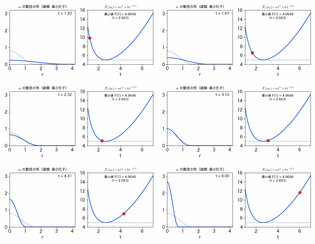
3 は**ビリアル定理**にあたり、最小化子では運動エネルギーと罰金の比が $3:4$ に決まります。数値は §7 で区間演算により $F[1]=4.96461575249750436315\ldots$ と確定します。最小化子の台の半径は $x_1/t_*\approx1.687$ です。

<Figure caption="最適化子の拡大縮小の族 u_t（L² ノルム 1）を動かしたときの 𝓔₁(u_t) = a t² + b t^{−3/2}。t = t* ≈ 2.663 で最小値 F[1] ≈ 4.9646 をとる。">
<img src="/figures/nash-dilation-energy.gif" alt="左は最適化子の動径の形が拡大縮小で細く高く、あるいは低く広く変わる様子。右は横軸 t、縦軸エネルギーのグラフで、赤い点が曲線の上を動き、t ≈ 2.66 の谷底で最小値 4.9646 を通過する。" loading="lazy" />
</Figure>

<Corollary id="cor-mf-subadditive" title="質量の分割の損">
$\theta_j\ge0$（$j\in J$、$J$ は可算）、$\sum_j\theta_j=\theta\lt\infty$ とすると $\sum_j\theta_j^{5/7}\ge\theta^{5/7}$ で、等号は $\theta_j\ne0$ となる $j$ が高々 1 つのときに限る。したがって $\gamma\gt0$、$\theta_1,\theta_2\gt0$ について
$$
E_{\mathrm{MF}}(\theta_1+\theta_2;\gamma)\lt E_{\mathrm{MF}}(\theta_1;\gamma)+E_{\mathrm{MF}}(\theta_2;\gamma) .
$$
</Corollary>

<Proof of="cor-mf-subadditive">
$\theta\gt0$ としてよいです。$\theta_j\gt0$ なら $\theta_j\le\theta$ から $\theta_j^{5/7}=\theta_j\theta_j^{-2/7}\ge\theta_j\theta^{-2/7}$ で、等号は $\theta_j=\theta$ のときに限ります。足すと $\sum_j\theta_j^{5/7}\ge\theta\cdot\theta^{-2/7}=\theta^{5/7}$ で、等号には $\theta_j\gt0$ の全ての $j$ で $\theta_j=\theta$、すなわちそのような $j$ が 1 つだけであることが必要です。後半は <Ref to="prop-mf-scaling" /> の 1 と前半からです。
</Proof>

この系は、質量を 2 つの塊に分けると必ずエネルギーが上がることを言っています。逆に、エネルギーが最小値に近い関数は質量を分けられないはずで、これを定量化するのが Lions の集中コンパクト性の原理の考え方です。

<Figure caption="質量 θ に対する最小値 E_MF(θ; γ) の両対数グラフ。直線は尺度則 θ^(5/7) γ^(4/7) F[1]、点は動径関数を格子で離散化して直接最小化した値（数値。相対差は 3×10⁻⁵ で、離散化の誤差）。">
<svg viewBox="0 0 480 290" width="100%" role="img" aria-label="質量 θ に対する最小値 E を両対数で描いたグラフ。γ = 1 と γ = 4 の 2 本の直線は傾き 5/7 で平行で、数値最小化の 10 個の点が直線の上に乗っている">
  <line x1="60" y1="260" x2="445" y2="260" stroke="currentColor" stroke-width="1" />
  <line x1="60" y1="10" x2="60" y2="260" stroke="currentColor" stroke-width="1" />
  <g font-size="12" fill="currentColor">
    <text x="60" y="277">0.1</text><text x="244" y="277">1</text><text x="420" y="277">10</text><text x="448" y="264">θ</text>
    <text x="40" y="241">1</text><text x="34" y="126">10</text><text x="28" y="14">100</text>
  </g>
  <line x1="70" y1="256" x2="70" y2="260" stroke="currentColor" /><line x1="250" y1="256" x2="250" y2="260" stroke="currentColor" /><line x1="430" y1="256" x2="430" y2="260" stroke="currentColor" />
  <line x1="60" y1="237" x2="64" y2="237" stroke="currentColor" /><line x1="60" y1="122" x2="64" y2="122" stroke="currentColor" /><line x1="60" y1="7" x2="64" y2="7" stroke="currentColor" />
  <polyline fill="none" stroke="currentColor" stroke-width="1.5" points="70.0,239.1 430.0,74.8" />
  <polyline fill="none" stroke="currentColor" stroke-width="1.5" stroke-dasharray="6 4" points="70.0,199.6 430.0,35.3" />
  <g fill="var(--sl-color-accent)"><circle cx="70.0" cy="239.1" r="4" /><circle cx="155.9" cy="199.9" r="4" /><circle cx="250.0" cy="157.0" r="4" /><circle cx="335.9" cy="117.8" r="4" /><circle cx="430.0" cy="74.8" r="4" /><circle cx="70.0" cy="199.6" r="4" /><circle cx="155.9" cy="160.4" r="4" /><circle cx="250.0" cy="117.4" r="4" /><circle cx="335.9" cy="78.2" r="4" /><circle cx="430.0" cy="35.3" r="4" /></g>
  <g font-size="13" fill="currentColor">
    <text x="300" y="150">γ = 1</text><text x="250" y="95">γ = 4</text>
    <text x="80" y="40">直線: θ^(5/7) γ^(4/7) F[1]</text><text x="80" y="58" fill="var(--sl-color-accent)">点: 数値最小化</text>
  </g>
</svg>
</Figure>


## 7. 計算機援用：$x_1$・$C_{\mathrm N}$・$F[1]$ の包含

$C_{\mathrm N}$ と $F[1]$ は $x_1$ と $\pi$ の初等的な式なので、$x_1$ を幅の狭い区間に閉じ込めれば、区間演算の包含原理によって定数も区間に閉じ込められます。ここでは mpmath（Python の多倍長演算ライブラリ）の区間演算 `iv` を 2 進 200 桁で使います。この節に限り、計算機援用の命題のために mpmath を使います。

```python
# Python 3.9.6, mpmath 1.3.0
from mpmath import iv, mp

iv.prec = mp.prec = 200          # 有効 2 進 200 桁

def g(x):                        # g(x) = sin x - x cos x（tan x = x と同値な形）
    return iv.sin(x) - x * iv.cos(x)

# 1. 二分法: g は [4.4, 4.6] で減少（g'(x) = x sin x < 0）なので、
#    区間で評価した g(m) の符号で根の側が確定する
lo, hi = mp.mpf('4.4'), mp.mpf('4.6')
assert g(iv.mpf(lo)).a > 0 and g(iv.mpf(hi)).b < 0
while hi - lo > mp.mpf(2) ** -180:
    mid = (lo + hi) / 2
    gm = g(iv.mpf(mid))
    if gm.a > 0:
        lo = mid
    elif gm.b < 0:
        hi = mid
    else:
        break
X = iv.mpf([lo, hi])

# 2. 区間 Newton 法の 1 歩: N = m - g(m)/g'(X) が X に含まれれば X に根はちょうど 1 つ
m = iv.mpf((lo + hi) / 2)
D = X * iv.sin(X)                # g'(X) の包含（0 を含まない）
N = m - g(m) / D
print('N ⊂ X :', X.a <= N.a and N.b <= X.b, '  0 ∉ D :', D.b < 0)

# 3. 定数の自然な区間拡張
pi = iv.pi
F1 = iv.mpf(7) / 3 * (iv.mpf(3) / 10) ** (iv.mpf(3) / 7) * (3 * pi / 10) ** (iv.mpf(2) / 7) * X ** (iv.mpf(6) / 7)
CN = iv.mpf(5) ** (iv.mpf(5) / 3) / (iv.mpf(2) ** (iv.mpf(2) / 3) * 3 * X ** 2 * (4 * pi / 3) ** (iv.mpf(2) / 3))
F1b = iv.mpf(7) / 4 * (iv.mpf(2) / (3 * CN)) ** (iv.mpf(3) / 7)

def outward(v, d=30):            # 下端を切り下げ・上端を切り上げて小数 d 桁で表示
    w = v * iv.mpf(10) ** d
    lo, hi = int(mp.floor(w.a.a)), int(mp.ceil(w.b.b))
    fmt = lambda n: f'{n // 10**d}.{n % 10**d:0{d}d}'
    return f'[{fmt(lo)}, {fmt(hi)}]'

for name, v in [('x_1', X), ('C_N', CN), ('F[1]', F1), ('F[1] (C_N 経由)', F1b)]:
    print(f'{name:14s}', outward(v))
print('2 つの F[1] の区間は交わる:', F1.a <= F1b.b and F1b.a <= F1.b)
```

出力（1 秒以内）:

```
N ⊂ X : True   0 ∉ D : True
x_1            [4.493409457909064175307880927280, 4.493409457909064175307880927281]
C_N            [0.058514615956547452340471145872, 0.058514615956547452340471145873]
F[1]           [4.964615752497504363152959214062, 4.964615752497504363152959214063]
F[1] (C_N 経由)  [4.964615752497504363152959214062, 4.964615752497504363152959214063]
2 つの F[1] の区間は交わる: True
```

<Proposition id="prop-cap-constants" title="定数の包含（計算機援用）">
次が成り立つ。
$$
\begin{aligned}
x_1&\in[4.493409457909064175307880927280,\ 4.493409457909064175307880927281],\\
C_{\mathrm N}&\in[0.058514615956547452340471145872,\ 0.058514615956547452340471145873],\\
F[1]&\in[4.964615752497504363152959214062,\ 4.964615752497504363152959214063].
\end{aligned}
$$
</Proposition>

<Proof of="prop-cap-constants">
**$x_1$.** $[4.4,4.6]\subset(\pi,\frac32\pi)$ で、<Ref to="lem-root-x1" /> から $g_0$ はそこで狭義減少、零点は $x_1$ だけです。コードの $g$ は $g_0$ の自然な区間拡張で、外向き丸めの区間演算（<Ref to="mathematics/computer-assisted-proofs/floating-point-interval-arithmetic#def-machine-interval" />）で評価しています。$\sin$・$\cos$ は 1 点の区間で評価するので、ライブラリが真の値を含む区間を返す限り、包含原理（<Ref to="mathematics/computer-assisted-proofs/floating-point-interval-arithmetic#thm-inclusion" />、<Ref to="mathematics/computer-assisted-proofs/floating-point-interval-arithmetic#prop-machine-inclusion" />）から `g(iv.mpf(m))` は $g_0(m)$ を含みます。したがってループの間ずっと $g_0(\mathrm{lo})\gt0\gt g_0(\mathrm{hi})$ が保たれ、中間値の定理（<Ref to="mathematics/calculus/limits-and-continuity#thm-ivt" />）と零点の一意性から $x_1\in X=[\mathrm{lo},\mathrm{hi}]$ です。（コードの 2 は、区間 Newton 法（<Ref to="mathematics/computer-assisted-proofs/floating-point-interval-arithmetic#thm-interval-newton" /> の 2）で $X$ にちょうど 1 つの零点があることを独立に確かめるもので、上の結論には使っていません。）

**$C_{\mathrm N}$、$F[1]$.** <Ref to="thm-sharp-nash" /> の $C_{\mathrm N}$ の式と <Ref to="thm-mf-closed-form" /> の 1 の第 2 の式は、$x$ と $\pi$ についての四則と単調な冪関数からなる式で、`iv.pi` は $\pi$ を含む区間です。$x_1\in X$ なので、包含原理から計算した区間 `CN`、`F1` はそれぞれ $C_{\mathrm N}$、$F[1]$ を含みます。表示は下端を切り下げ、上端を切り上げているので、表示した区間も真の値を含みます。
</Proof>

<Remark id="rem-cap-assumption" title="計算機援用の前提と検算">
この命題が仮定しているのは、mpmath の区間演算が外向き丸めを正しく実装し、`iv.sin`・`iv.cos`・`iv.pi`・冪が真の値を含む区間を返すことです（計算機援用証明で通常置く前提）。独立な検算として、(1) $F[1]$ の 2 つの閉じた形（<Ref to="thm-mf-closed-form" /> の 1）が別々の式から計算されて同じ区間に入ること、(2) 倍精度の Brent 法で求めた $x_1=4.493409457909064$、$F[1]=4.964615752497503$ と一致すること、(3) §6 の図の直接最小化が $F[1]$ を相対誤差 $3\times10^{-5}$ で再現することを確かめています。
</Remark>

## 8. 演習

<Exercise id="exr-gauss-nash" difficulty="易">
$f(x)=e^{-\lvert x\rvert^2}$（$x\in\mathbb R^3$）について $\lVert f\rVert_1$、$\lVert f\rVert_2^2$、$\lVert\nabla f\rVert_2^2$ を計算し、$\mathcal N_3(f)=\frac1{6\pi}$ を確かめよ。
<Solution>
$\int e^{-\alpha\lvert x\rvert^2}dx=(\pi/\alpha)^{3/2}$、$\int\lvert x\rvert^2e^{-\alpha\lvert x\rvert^2}dx=\frac3{2\alpha}(\pi/\alpha)^{3/2}$ です。$\lVert f\rVert_1=\pi^{3/2}$、$\lVert f\rVert_2^2=(\pi/2)^{3/2}$、$\lvert\nabla f\rvert^2=4\lvert x\rvert^2e^{-2\lvert x\rvert^2}$ から $\lVert\nabla f\rVert_2^2=4\cdot\frac34(\pi/2)^{3/2}=3(\pi/2)^{3/2}$ です。よって
$$
\mathcal N_3(f)=\frac{(\pi/2)^{5/2}}{3(\pi/2)^{3/2}\pi^2}=\frac{\pi/2}{3\pi^2}=\frac1{6\pi}\approx0.0531
$$
で、$C_{\mathrm N}$ との比は $0.907$ です。
</Solution>
</Exercise>

<Exercise id="exr-nash-exponents" difficulty="標準">
定数 $C$ と実数 $p,q,r$ について、すべての $f\in C_c^\infty(\mathbb R^d)$ で $\lVert f\rVert_2^p\le C\lVert\nabla f\rVert_2^q\lVert f\rVert_1^r$（$f\ne0$）が成り立つとする。$f$ を $\lambda f(\mu\,\cdot)$ に置き換えることで、$q=2$ と正規化したとき $p=2+\frac4d$、$r=\frac4d$ に限ることを示せ。
<Solution>
$f_{\lambda,\mu}=\lambda f(\mu\,\cdot)$ では $\lVert f_{\lambda,\mu}\rVert_2=\lambda\mu^{-d/2}\lVert f\rVert_2$、$\lVert\nabla f_{\lambda,\mu}\rVert_2=\lambda\mu^{1-d/2}\lVert\nabla f\rVert_2$、$\lVert f_{\lambda,\mu}\rVert_1=\lambda\mu^{-d}\lVert f\rVert_1$ です。不等式の両辺の比が $\lambda,\mu$ によらず有界であるためには、$\lambda$ の冪について $p=q+r$、$\mu$ の冪について $-\frac d2p=(1-\frac d2)q-dr$ が必要です（そうでなければ $\lambda$ か $\mu$ を $0$ か $\infty$ に送って不等式が破れる）。$q=2$ とすると $p=2+r$、$-\frac d2(2+r)=2-d-dr$ から $r=\frac4d$、$p=2+\frac4d$ です。
</Solution>
</Exercise>

<Exercise id="exr-support-radius" difficulty="標準">
$E_{\mathrm{MF}}(\theta;\gamma)$ の最小化子 $\sqrt\theta\mu^{3/2}u_*(\mu\,\cdot)$（<Ref to="prop-mf-scaling" />・<Ref to="thm-mf-closed-form" />）の台の半径 $\mathcal R(\theta,\gamma)$ を求め、$\theta$ と $\gamma$ への依存を述べよ。
<Solution>
$u_*$ の台の半径は $x_1/t_*$ で、$\sqrt\theta\mu^{3/2}u_*(\mu x)$ の台の半径はその $\mu^{-1}=\gamma^{-2/7}\theta^{1/7}$ 倍です。よって $\mathcal R(\theta,\gamma)=\frac{x_1}{t_*}\theta^{1/7}\gamma^{-2/7}\approx1.687\,\theta^{1/7}\gamma^{-2/7}$ です。質量を増やすと台はゆっくり（$\theta^{1/7}$）広がり、罰金 $\gamma$ を強めると狭まります。最小化子の高さ $\sqrt\theta\mu^{3/2}u_*(0)$ は $\theta^{2/7}\gamma^{3/7}$ に比例します。
</Solution>
</Exercise>

## 参考文献

- J. Nash, "Continuity of solutions of parabolic and elliptic equations", *American Journal of Mathematics* 80 (1958), 931–954.
- E. A. Carlen, M. Loss, "Sharp constant in Nash's inequality", *International Mathematics Research Notices* 1993, no. 7, 213–215. [doi:10.1155/S1073792893000224](https://doi.org/10.1155/S1073792893000224)
- E. H. Lieb, M. Loss, *Analysis*, 2nd ed., American Mathematical Society, 2001 — 第 3 章（再配置）、第 7・8 章（勾配と Sobolev の不等式）。
- P.-L. Lions, "The concentration-compactness principle in the calculus of variations. The locally compact case, Part I", *Annales de l'Institut Henri Poincaré, Analyse Non Linéaire* 1 (1984), 109–145.
- V. Bach, A. Hach, "On the ultraviolet limit of the Pauli–Fierz Hamiltonian in the Lieb–Loss model", *Annales Henri Poincaré* 23 (2022), 2207–2245. [doi:10.1007/s00023-021-01124-2](https://doi.org/10.1007/s00023-021-01124-2)
- W. Tucker, *Validated Numerics: A Short Introduction to Rigorous Computations*, Princeton University Press, 2011.